![]()
In analyzing the variable distribution within a solution, it is quite helpful to look at some type of Probability Density Function for the variable. There are a few interpretations of this function depending upon whether you are looking at the probability across time, space, or different datasets. In essence, the spatial probability density function indicates to the engineer how much of the domain (% of total volume in this case) which contains particular variable range. “How much of the domain has Species 1 near 0.01, or How much of the domain has Temperature near 900 degrees K”.
This particular tool I wrote is to analyze the distribution of a function spatially, sometimes referred to a volumetric probability density function, or a volumetric histogram. In a very basic interpretation, it is similar to the histogram display in the Color Palette Editor, normalized based on element volume.
This routine takes the parent part(s) that you have selected along with the variable that you would to interrogate, and a user specified number of bins (or bars) in the histogram. The routine automatically finds the minimum and maximum variable range for the part(s). Based on this range, it then divides the volume into N number of IsoVolumes (number of bins) based on this variable range. The routine then determines the fraction of the total volume which is contained within each of these variable constrained ranges. The result is placed into a query register and automatically plotted on the screen.
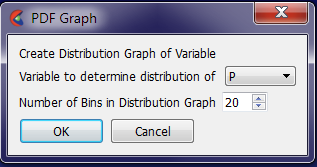
The Tool presents the user with the simple Window to select the variable, and number of bins (or bars) for the distribution function.
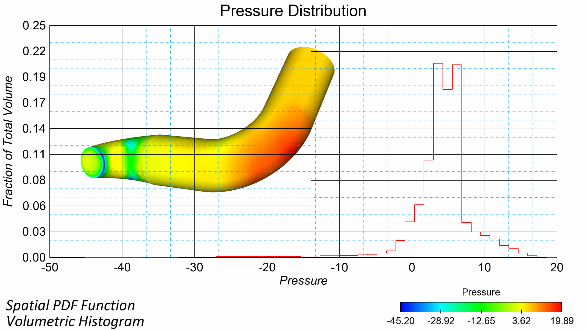
After executing, you will then get a graph of distribution of the variable within the parent part(s) selected.
The values on the graph should always sum to 1.0, as it is presented as a fraction of the domain which contains that variable.
Note: As users increase the number of bars( or bins) for the graph, the shape of the curve will increase in resolution, although values on the Y-axis of the graph will adjust (as more bins used will still sum to 1.0).
Update 16-April-2012:
Based on User Requests, the routine has been updated to create a Stair-Stepped Graph rather than the smooth graph to represent the “binning” concept further in the graph.
Updated 22-April-2012:
Based on User Requests, the routine has been updated to handle transient models now. It does this by exporting out each timestep as a 1D bar part that is then automatically read back into EnSight at the end. This results in the PDF function correctly sitting in the time domain, and allows the user to normally control the timestep & all other features of EnSight while the PDF Graph correctly dove-tailed into the hierarchy of EnSight. This also allows the user to further interrogate and and operate with the data as though it were normal Elemental Data (filtering, elevated surfaces, coloring, etc.)
I also updated the routine to correctly work with 2D parent parts (using the EleSize() and StatMoment() together rather than Vol().)
In addition, I also updated the routine to select the original Parent Parts for ease of repeat usage (rather than leaving the IsoVolume part selected).
Here is a example movie made from the Transient PDF function:
Update 05-Nov-2013:
Updated routine for bug regarding the variable used for the IsoVolume. Previously, the variable selected in the GUI might not have been the variable used in the IsoVolume. Fixed in version 2.3
Update 03-Nov-2015 :
Updated the explicit setting for the IsoVolume to “Band”, rather than default (not explicitly set). This would cause problems if previous IsoVolumes were not of type == Band.
Full Change log within header of Python File